December 2017 – Insights From A Quant

Trend-following Bitcoin

December 21, 2017 by Kent Peterson

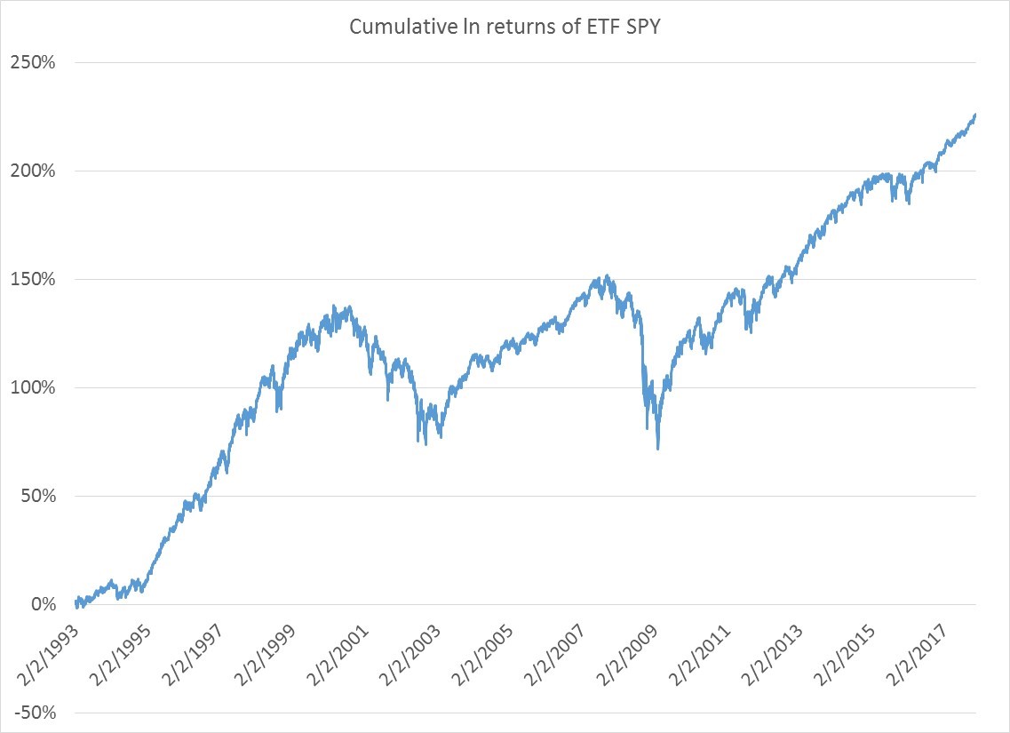
Bitcoin, along its blockchain brethren, is an interesting, relatively new instrument that has emerged from utter obscurity. When two different exchanges are rushing to launch a new financial future, a hedge fund you interviewed with has abandoned its other investments to focus solely on bitcoin, and governments are shutting off access to a market, you know a market is HOT, but also not fully understood or trusted. Whether crytpocurrencies are in the long-run a legitimate alternative to sovereign currencies or centuries old stores of value like gold and silver is another question. It is, as many new technologies and instruments are prone to be, an object of intense speculation. Calling this is a bubble or a mania is semantics. Gauging the levels of dumb money or retail participation is difficult because of the lack of centralized exchange and public information about who is buying. Nevertheless, the price swings are huge, and the historic losses have been awful. But if you were an early investor, or miner who held on, the rewards were incredible.

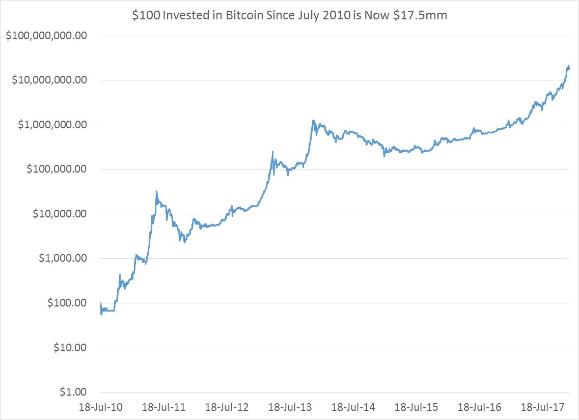
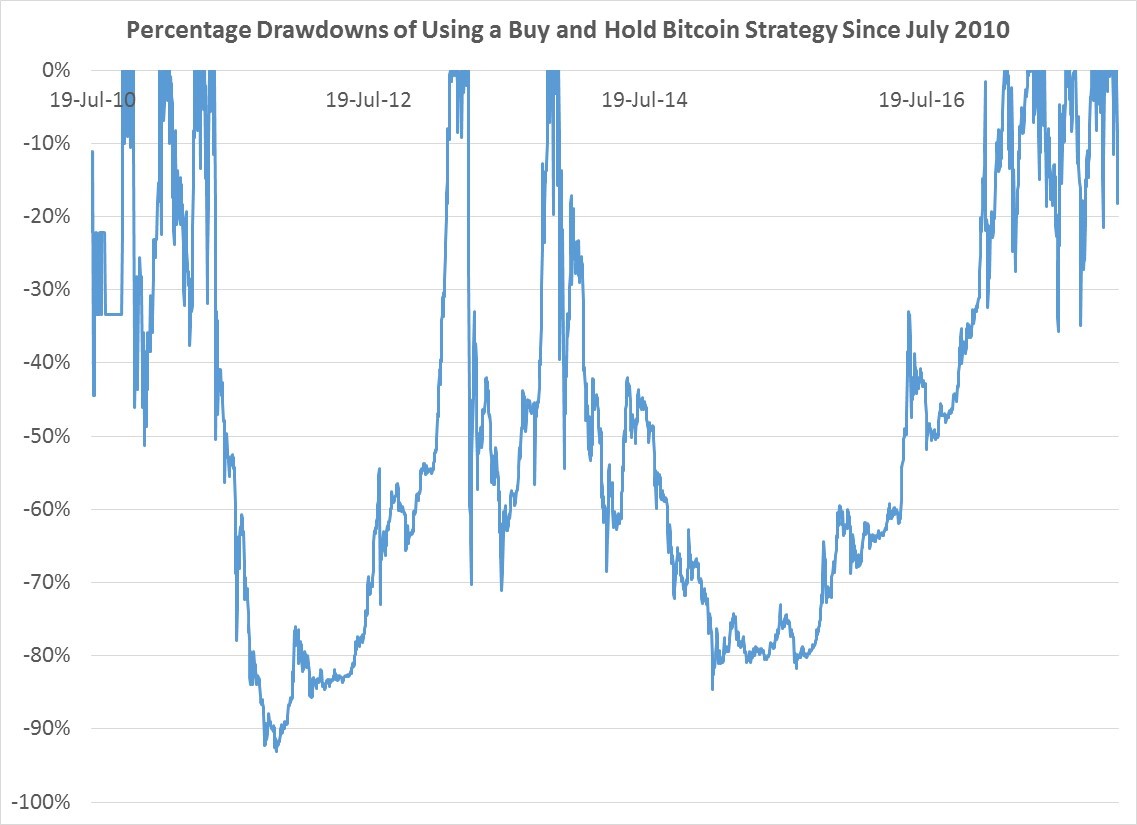
But those returns, shown in the chart above, assume you stood the course, because it was a rough, rough ride as you can see in the next chart. Losses of 80% and 90% of your investment were simply the norm. Expect the same in future.

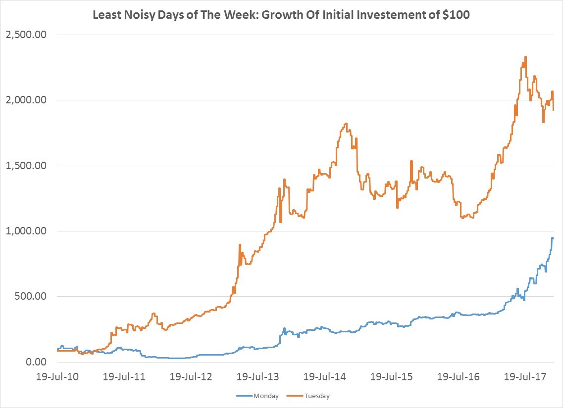
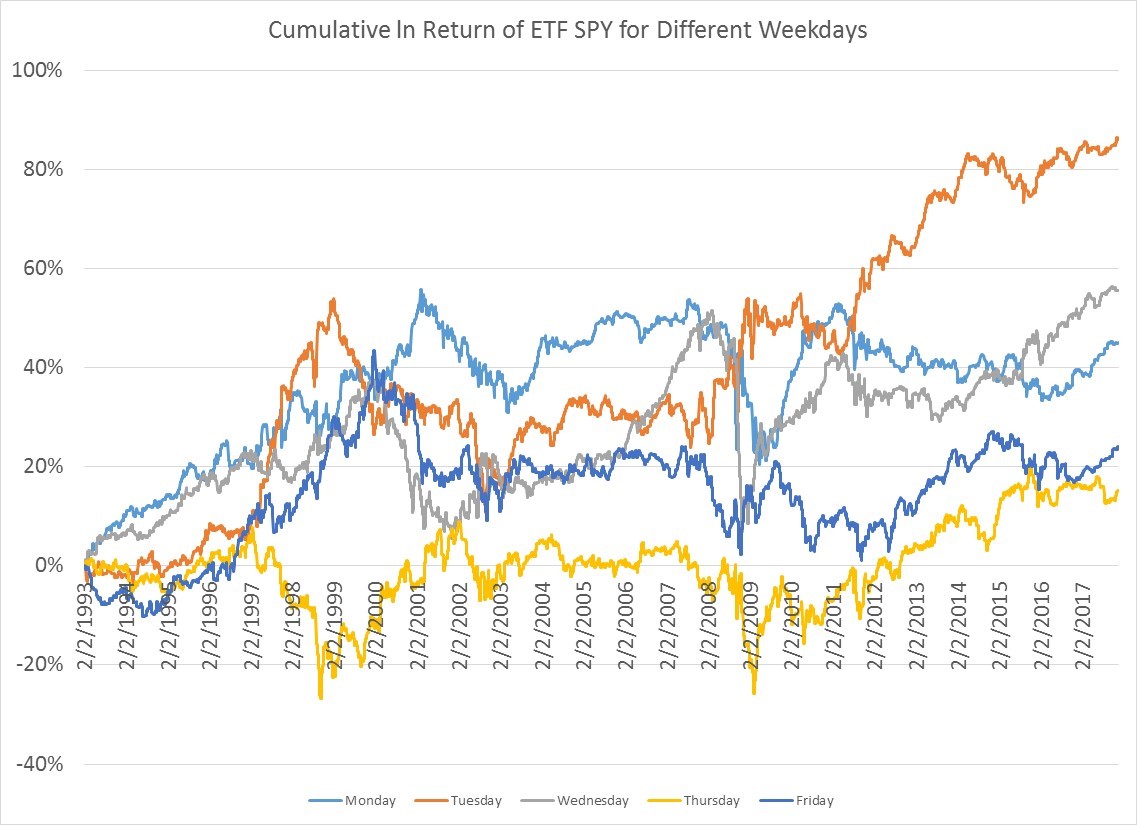
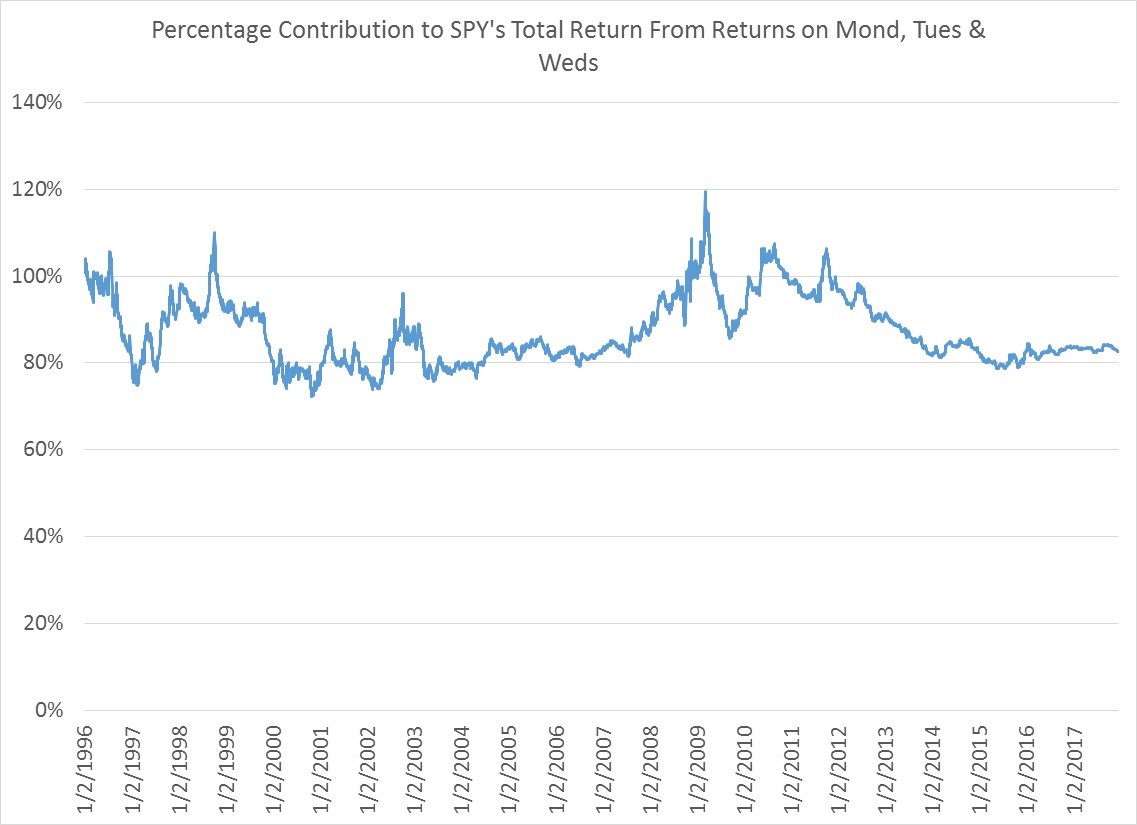
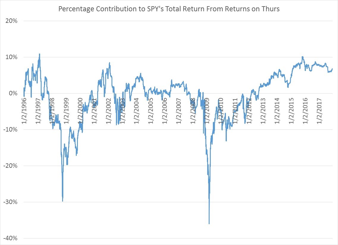
Since there is little data at this point, we don’t really have enough sample size to get any meaningful numbers on monthly seasonality. When you dig into daily seasonality, you don’t see a ton either. Its noisy, though as you can see in the next chart, Tuesdays and to larger extent Mondays have tended to be days that Bitcoin goes up most consistently.

One thing Bitcoin does do consistently is trend, so an investor may consider a tactical timing strategy built around some such rules. The rules applied below were as follows: buy bitcoin if it has been up over the last 250 days, and for the first year when 250 days were not available, buy it if Bitcoin is up over the last month, otherwise don’t hold bitcoin. This turns out to have worked a lot better than buy and hold strategy, since your $100 would be worth $31 million dollars instead of a paltry $17.5 million.

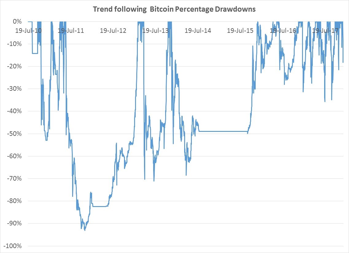
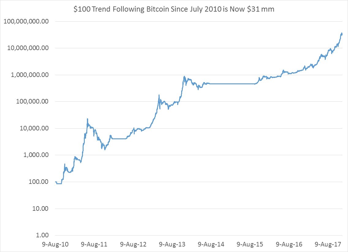
And the ride on the downside, while less horrific than a buy and hold strategy, was still rather violent and scary since you still lose 90% of your money at one point.

Whether Bitcoin will continue to soar and offer buy and hold investor or trend followers the same spectacular returns is unknown. What seems certain is the volatility of 79% annualized will probably be the norm for awhile.

Please follow and like us:

The Odd Weekday Seasonality of SPY: Avoid Thursdays and Fridays

December 14, 2017 by Kent Peterson

There is an old investing adage: “Sell in May and go away,” perhaps created by those who kept their yachts in Newport and wished to summer care free from the vagaries that the stock market brought from June until October. While I lack the poetic wherewithal to create an adage that rhymes and is catchy, there has been a similar kind of under-performance factor in the ETF SPY since since its inception in 1993. Thursday and Friday have offered the investor weak and sub-par returns relative to Monday through Wednesday. Most long only equity traders would be better heading to the beach, gym or golf course on Thursdays in particular.

Below is a cumulative natural log chart of the ETF SPY since its inception in 1993. Two bear markets and one long bull market recently.

The next chart shows the cumulative ln returns of holding SPY close to close on all five weekdays. That chart by itself doesn’t tell you that much other than that trading any one weekday is a bit noisy.

Its when you group days together that the story gets interesting. Below you can see how much of SPY’s positive return through time has come from the first three days of the week on a percentage contribution basis. The way to read this chart is simple: if the SPY gained 100% cumulatively over a 15 year period a reading of 95% would indicate that 95% of the total 100% cumulative return came from M-W and only 5% from Thurs and Friday. As you can see, over the past few years 83-84% of the cumulative returns for SPY since 1993 has come from Monday, Tuesday and Wednesday. At times, because other weekdays like Thursday and Friday were net detractors from cumulative returns, their contribution actually has exceeded 100%, especially during the financial crisis.

Finally, if you believe in day of the week seasonality, you should close up shop Wednesday night go away on Thursday. As you can see in the final chart, Thursdays detracted massively from SPY’s cumulative returns during the last 2 bear markets. Historically only 7% of SPY’s cumulative positive returns since 1993 have come from Thursdays.

Please follow and like us:

Volatility Targeting An Equity Index

December 11, 2017 by Kent Peterson

Volatility Targeting is a simple concept. You set an annual volatility target for an asset, and adjust your exposure through time to meet that target. If your annual vol target is 10% and your measure of the asset’s volatility is 20%, you would hold 50% (10 divided by 20) of the asset to achieve the 10% vol. Mathematically, your vol target is the numerator and your denominator is the vol estimate. Most people either use implied volatility or trailing historic volatility as their vol estimate. The question arises: why bother?

Well this concept is to a large degree second nature in hedge fund portfolios where it is a necessity. If you have equal conviction that 2 year Note futures and S&P 500 futures are going to rise, you want them to have an equal impact on your PL. Buying equal dollar amounts of both is pretty dumb, because all the volatility in your portfolio will come from the equity future position. You have to either bring up the vol of your 2 year Note position to equal your S&P future position, or dial your equity down. Vol targeting enables greater diversification by allowing uncorrelated assets to have the same impact in a portfolio. This is the core idea behind risk-parity portfolios which use multiple assets.

In the last 10-15 years, this concept has entered into mainstream portfolio management. And with good reason. It works, though its popularity or overuse are now its biggest danger. In general, the version employed in Mutual Fund and ETF land is more constrained—hedge funds don’t have an issue leveraging up 2 year notes 20 times or more to be at the same vol as the S&P 500. Long only mutual fund managers are wary of levering anything more than 150%. There are more regulations and leverage is “bad optics,” as I once heard someone say. It is also within mainstream portfolio management that the idea has been applied more consistently to a single asset class, mostly equities, to be a tactical allocation decision device: putting more money into equities when equity vol is low, and less when vol is high.

Using the SPY ETF, shows the performance enhancements and side effects that come from the vol target pharmacy when applied to a single asset.

For our exercise we will examine the performance of two portfolios, the ETF SPY and our volatility target enhanced version of the same. Our volatility target is 1% daily vol or 15.8% annualized. Our vol estimate will use the trailing standard deviation of SPY over the last 200 days as the denominator. We can have a maximum position or leverage cap of 150% invested. We will rebalance every Monday at the close.

Below is the PL from both portfolios. Over time both portfolios do well, but the volatility target version offers better total returns.

Here are the performance stats. When you look at risk-adjusted returns, the vol target portfolio is superior when you consider either the ratio of return to volatility or max loss.

	SPY	SPY Vol Tgt
Annual % Return	10.8%	12.1%
Annual Vol	19%	16%
Info Ratio	0.58	0.74
Max % Drawdown	-55%	-39%

The vol target version of SPY experienced less painful maximum losses during the bear markets of 2003 and 2008.

The last chart, and perhaps the most interesting, shows the relative out performance of the vol target strategy vs. SPY alone through time. What is apparent is that while it works, there are times when the vol target version of SPY really under-performs. Vol target SPY has been brilliant from 2012 to present as volatility has just gone to sleep and you are levering up in a bull market. The strategy also performed as designed going into the 2008 crisis, cutting risk as equities tanked. But consider the equity bubble in 1998 and 1999 when stock returns were incredible, but vol itself was very high and you dialed back your equity exposure. In this period you would have been much better off just buying SPY. The post 2008 crisis period was also terrible. Your trailing vol estimate combined with higher vol in general even in the implied vol market kept you dialed back in equities at a time that it would have been much better to just buy, and hold on for the ride. In a high vol, high return environs, vol targeting can look pretty bad.

Please follow and like us:

An Intraday Oddity in VIX Futures

December 8, 2017 by Kent Peterson

One of the odder facets of capital markets in the last few years has been the shockingly low level of volatility, both realized and implied, especially in equity markets. Coincident with this decline in the level of volatility has been the emergence of two parallel developments.

Huge swathes of money, especially in equities, are now allocated completely mechanically on the basis of level of the VIX or historical realized volatility, whether in guaranteed annuities or risk parity portfolios. As a tactical strategy, this backtests well: if you cut your equity risk when vol rises, and vice-versa, you end up with decent returns, especially around crises. The problem is that everyone knows this now, and it’s a crowded trade. At some point in the future, some large and unexpected spike in volatility will cause these portfolios to liquidate equities en masse in a “portfolio insurance” herding a la the 1987 crash. And then someone will scapegoat the quants who developed and used these asset allocation models.

Second, volatility has now emerged as an asset class in its own right, with liquid securities from ETFs to VIX futures offering traders a path to express their view on the future direction of vol itself. Whether or not implied volatility in equities should be viewed as an asset class in itself is pretty dubious, given its high negative correlation to equities: if you are long stocks and short vol, you have increased the risk in your portfolio. Nevertheless, this is a radical change from even fifiteen years ago when someone who wanted to express a view on US equity vol had to buy or sell a straddle or strangle and every day manage the delta of her position. By comparison, it’s a cleaner, cheaper and simpler world today if you are a vol trader: just buy or sell a VIX future…done.

Shown below is the VIX Index since Dec 2016. Vol has moved downward in a random scary pattern from 14 to 10. Being short vol for this whole time was a successful, albeit painful & noisy trade.

To be clear, you can’t trade the VIX itself, only ETFs derived from it or VIX futures, which are probably the cheapest way to get equity vol exposure. The VIX futures curve is “typically” upward sloping as you move out the curve with contracts farther from expiry trading at higher prices. Over time this means that there is a roll-down effect from the natural term-structure: a contract that starts off at a price of say 15 three months from expiry will “roll down” closer to 12 as it approaches expiration, and the contract trading closest to expiry will converge downward towards the cash VIX Index itself. So there is a natural tendency for VIX contracts to fall or lose value over time in a stable or normal market environment. The VIX futures curve can invert and do lots of contortions in a market crisis, but that is another blog post.

Let’s say you were looking for a more consistent way to trade both the decline in the VIX over the last year and capture the tendency of VIX futures to decline over time. You could simply buy farther dated VIX futures and hold them until expiry, but this would give you a pretty bumpy ride.

Maybe you were looking for a more consistent and less risky way to make money being short vol over this time? So you investigated day trading VIX futures. If you were observant you would have noticed the following.

If you shorted the first VIX future every day from 8:30 am to 8:30 PM, ignoring transaction costs, you would do OK PL-wise, but its still a noisy path.

And if you did the complete opposite, and decided to short the first VIX future every night at 8:30 PM and cover your short at 8:30 am before the chaos of US economic announcements hits your position, again ignoring transaction costs. Well that works much better.

Why is this occurring? I don’t know, some of it is attributable to a bull market, but its strikingly persistent and weird pattern/anomaly. And it really doesn’t make much sense that the decline in Vol would happen in such a consistent part of the day, but there it is. The contrast between the random noise of the intraday vol down move vs the overnight decline is quite stunning. How long it will continue is anyone’s guess.

Please follow and like us:

A Better Blend: Stock, Bond and Managed Futures

December 8, 2017December 5, 2017 by Kent Peterson

Assume its 1984, and you have 3 investment choices in front of you:

Stocks: Buy the S&P 500 Index and pay 50 bps in fees per annum.
Bonds: Perpetually buy 10 year bonds and pay 30 bps in fees a year.
Managed Futures: Build a trend following portfolio around 4 futures contracts: S&P 500 futures, 30 Year Bond futures, Crude Oil Futures and US$ futures, since each represents a different asset class. At each month-end, for each of the 4 contracts, you go long a contract when its 1 year trailing return is positive, and short when it is negative. Equalize the risk of all 4 contracts, and penalize your returns by a) assuming you pay 1% a year in commissions, rolls and fees, and b) ignore your return on the cash that is not being held as margin, which up until recently considerably boosted your returns.

The simple portfolio of investing 50% of your money in stocks and 50% in bonds turns out to be quite attractive over the last 30+ years. Your returns are only 0.8% lower than if you had held equities alone, because long maturity yields fell dramatically over this period, so your equally blended portfolio achieves almost the same return with a fraction of the risk, whether you define risk as annual standard deviation (volatility) or maximum % loss.

The only real drawbacks to this portfolio are a) going forward your bond returns (at current low yields) are extremely unlikely to be this high, and b) at some point along the investment path, you still can expect to lose 25% of your money.

	S&P 500	10 Year Bond	50/50 Port
Avg Annual % Return	8.9%	7.3%	8.1%
Annual Volatility	14.8%	7.8%	8.3%
Return to Vol Ratio	0.60	0.93	0.98
Maximum % Drawdown	-54%	-11%	-25%

This is the 50/50 portfolio compared to equities alone.

This is the max percentage drawdown or loss you would experience in each portfolio.

Consider adding the third strategy, which only requires trading once a month. First compare the performance stats of all three strategies over the last 33 years in isolation. A simple managed futures strategy has volatility and returns that fall between stocks and bonds, and a return to risk (or information ratio) between the two asset classes (with drawdowns slightly worse than bonds alone).

	S&P 500	10 Year Bonds	Mngd Futs
Avg Ann % Return	8.9%	7.3%	8.0%
Annual Volaility	14.8%	7.8%	11.2%
Return to Risk Ratio	0.60	0.93	0.71
Max % Drawdown	-54%	-11%	-18%

Putting the 50/50 portfolio side by side with a portfolio that puts 1/3^rd in each strategy, an investor ends up with pretty much the same return, but the risk, as measured by volatility improves, while your max percentage loss is cut in half from -25% to -12%.

	50/50	1/3rd Each
Avg Ann % Return	8.1%	8.0%
Annual Volatility	8.3%	7.3%
Return to Risk Ratio	0.98	1.10
Max % Drawdown	-25%	-12%

Below is a chart of the two portfolios cumulative returns through time. You start and end up in virtually the same place, but the ride is a lot smoother.

And the two max % drawdowns in the portfolios.

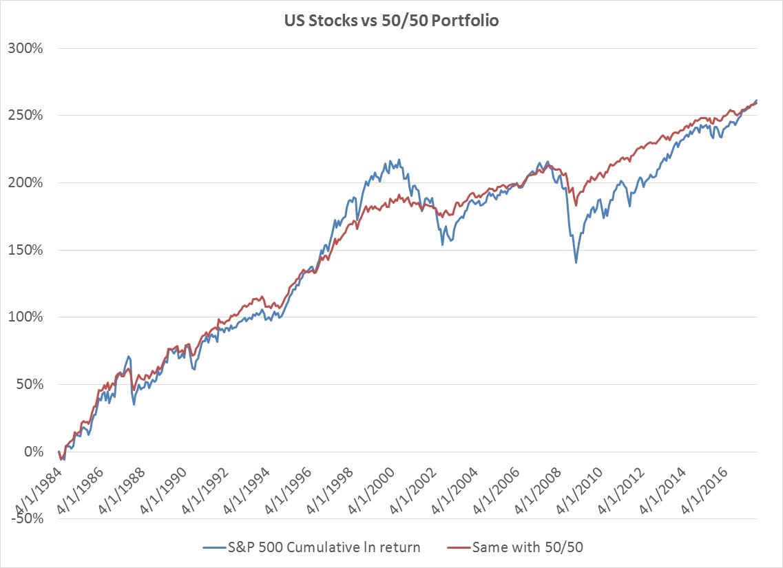
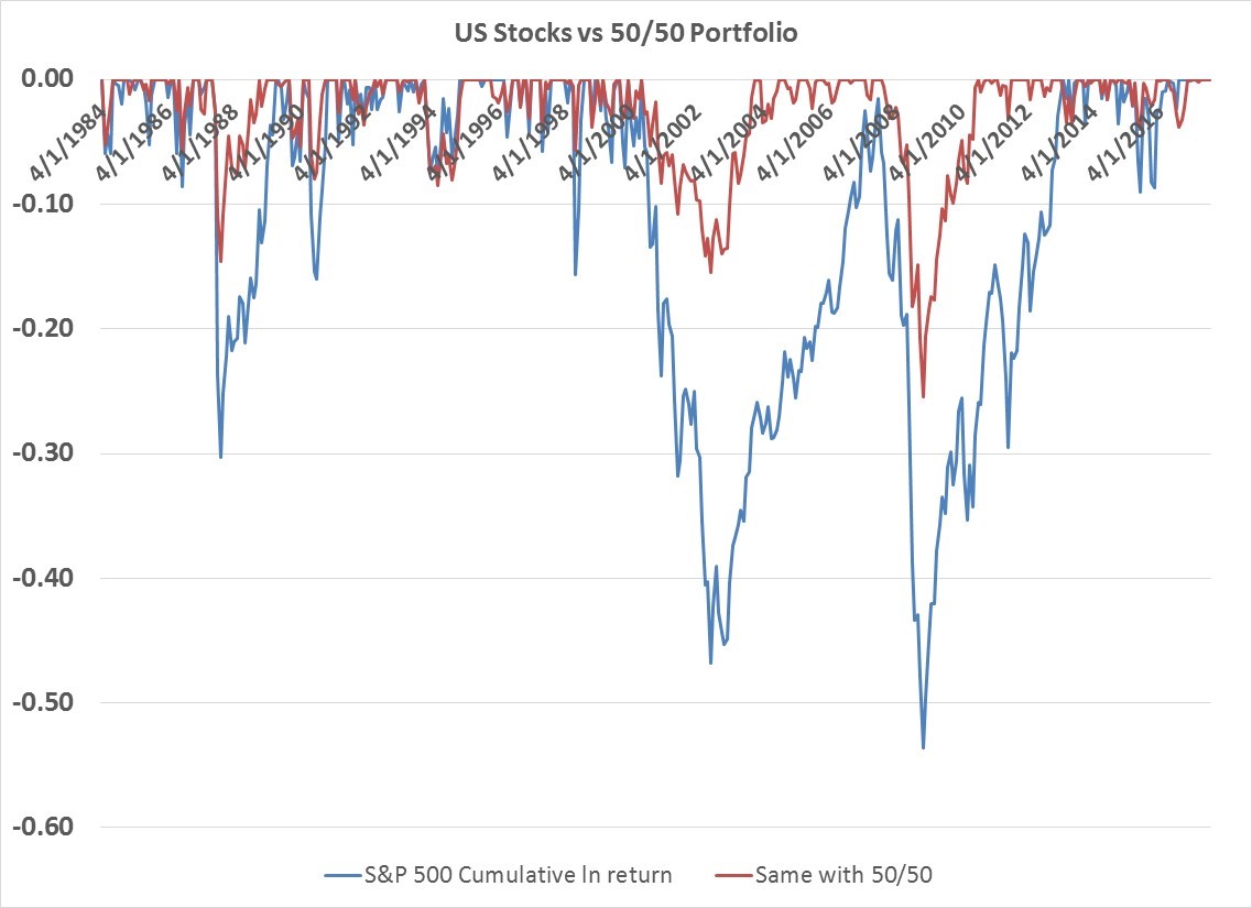
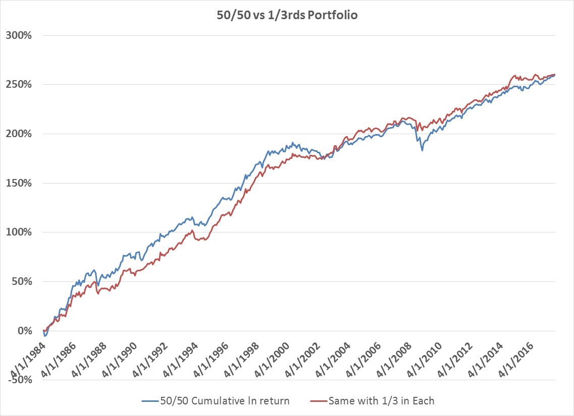
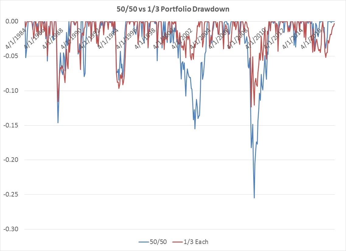
There are other ways of slightly improving the portfolio blend—you could add more than 4 futures to your managed futures strategy for further diversification. Similarly, a risk parity version of the 1/3 portfolio that equalizes volatility among all 3 strategies improves your risk-adjusted returns and brings your max % loss down to -10.4% from -12.4%.

But all this is making a simple message more complicated—the value added from a managed futures allocation, whether you DIY or outsource it is huge. The only free lunch in investing is diversification, and managed futures are a huge diversifier. The simplistic managed futures strategy simulated here has a 0.10 correlation to US stocks and 0.28 correlation to 10 Year Treasury returns. Managed futures can and will have periods where returns are unflattering when viewed in isolation. But that’s missing the point. Investors should seek out multiple return streams with positive expected return over a reasonable time horizon that diversify their portfolios and blend them together. Managed futures fit this diversification role perfectly.

Please follow and like us: